Introduction
Filter design using Eigenmodes and Eigenmode solvers is the subject of this page. Eigenmode analysis is concerned with the building blocks and sub-structures of a distributed element filter. The Eigenmode Solvers of CST or HFSS provide such analysis.
There are two major types of 3D electromagnetic (3D-EM) analyses for passive, non-radiating structures:
- driven modal analysis (excitation via waveports – energy is supplied to the structure from an external source – yields internal fields and port S-parameters)
- eigenmode analysis (no excitation – stored energy in the structure exists) – analysis in terms of internal fields for each mode, natural modes, resonances – no S-parameters)
The driven modal analysis involving ports and applied power sources is the more frequently used simulation type as it yields port S-parameter data which can also be measured at a physical prototype with relative ease. A defined field at a given port boundary is applied as excitation for the 3D EM structure and that excitation causes EM fields to build up in the structure and possibly propagate to other ports. The internal fields can be viewed in different formats. Reflection and transmission S-parameters are then derived from the field solution. This is clear and requires no further explanation.
Now what about that ‘Eigenmode’ stuff ?
Eigenmode solvers perform an ‘undriven’ analysis insofar as no external power source is involved and no waveports are used (except for the purpose of resistively loading a resonator in order to find the “loaded quality factor“). Instead, a certain amount of stored energy is assumed to be “trapped” in the structure and the Eigenmode solver reveals the resulting modes and their field properties. Once the fields and surface currents are known, finite conductivity can be applied and the resonator-Q is found via the relationship between stored energy and dissipated energy per cycle.
Eigenmode solver analysis is useful for resonator design and it also allows estimation of filter stopband behavior where the higher order modes of a resonator may limit the selectivity of a filter. Conveniently, a 2-resonator Eigenmode solver analysis can be used for the design of the couplings of coupled-resonator bandpass filters.
Mathematically: λ is an Eigenvalue of a square matrix A, if V x A = V x λ with V being a non-zero vector.
Most users of EM simulation software who have used Eigenmode analysis will relate this analysis only to resonators and even the 3D EM software help file may highlight that Eigenmode solver analysis is intended for resonances and quality factors. While this is perhaps the main application – Eigenmode solver analysis is certainly not limited to resonances and Q’s.
Analysis of resonators
When we design a filter, the resonators are our building blocks. Surely, we want to know in advance what properties a particular chosen resonator can offer. Usually we want to also see the effect of conductivity of the internal surface material on the unloaded Q – the Q ultimately determines the passband insertion loss of a filter. Eigenmode analysis models consist of a 3D model of the proposed resonator. As an example, a TEM-mode coaxial resonator is shown below:

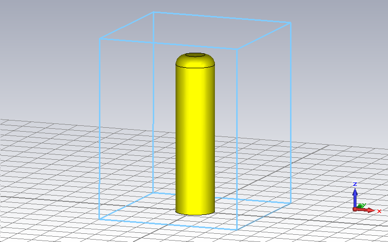
and in CST
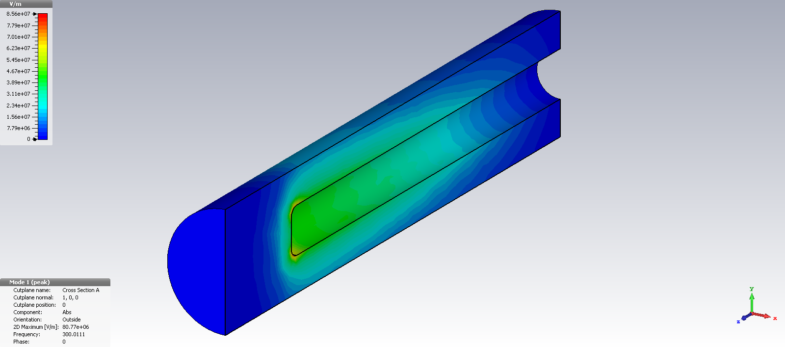
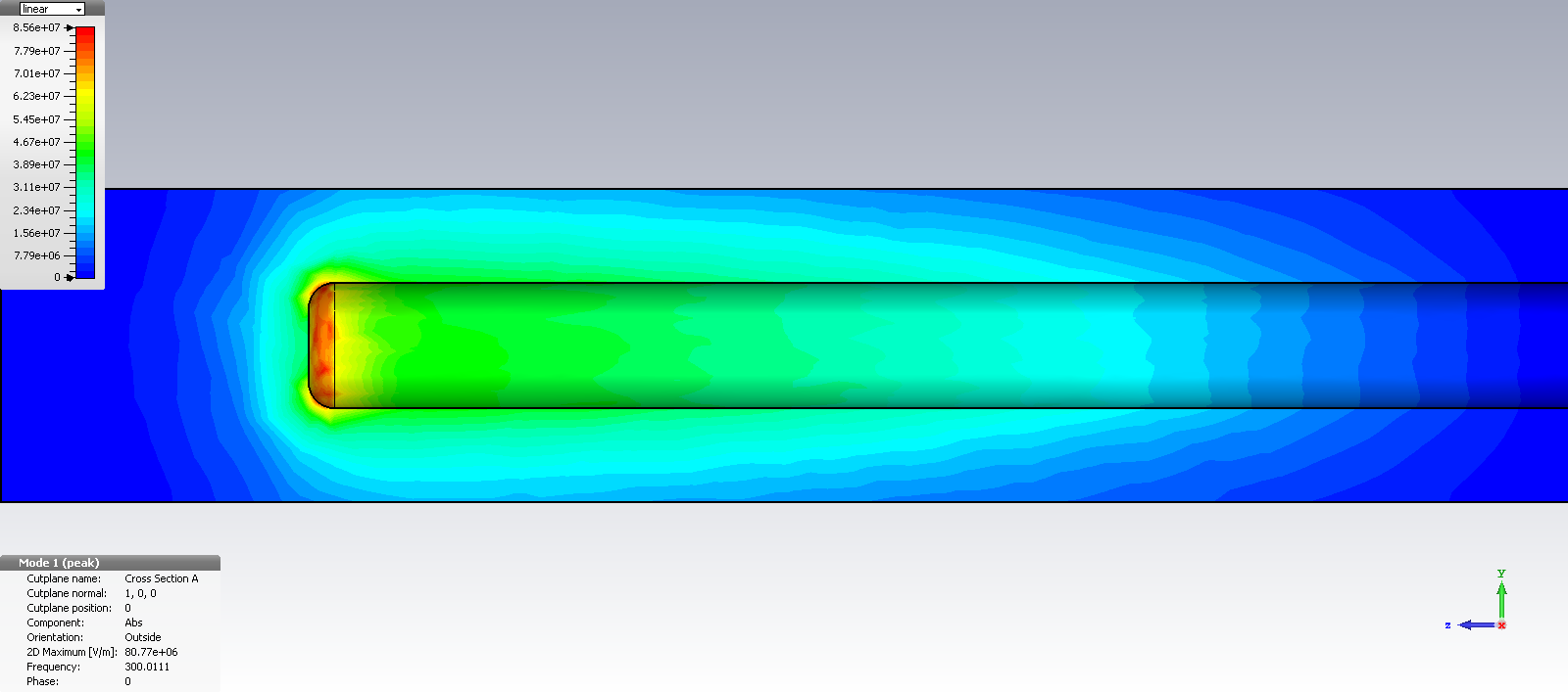
The Eigenmode solver can be set up to show multiple resonances (fundamental and higher order) and its associated unloaded Q-factors (if material with finite conductivity has been defined). Below images show a TEM-mode coaxial resonator and its fields at the fundamental quarterwave resonance obtained from CST Eigenmode analysis.
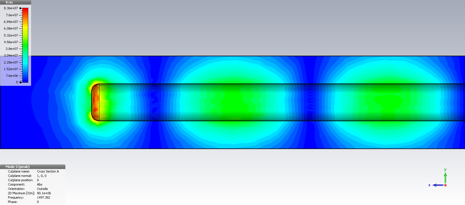
The next higher resonance occurs when the inner rod length is three quarterwaves long: l = 3/4*lambda. We can find the order of the resonance by E-field inspection. We clearly see one halfwave on the right side, followed by a quarterwave length with its Emax at the open end of the rod.
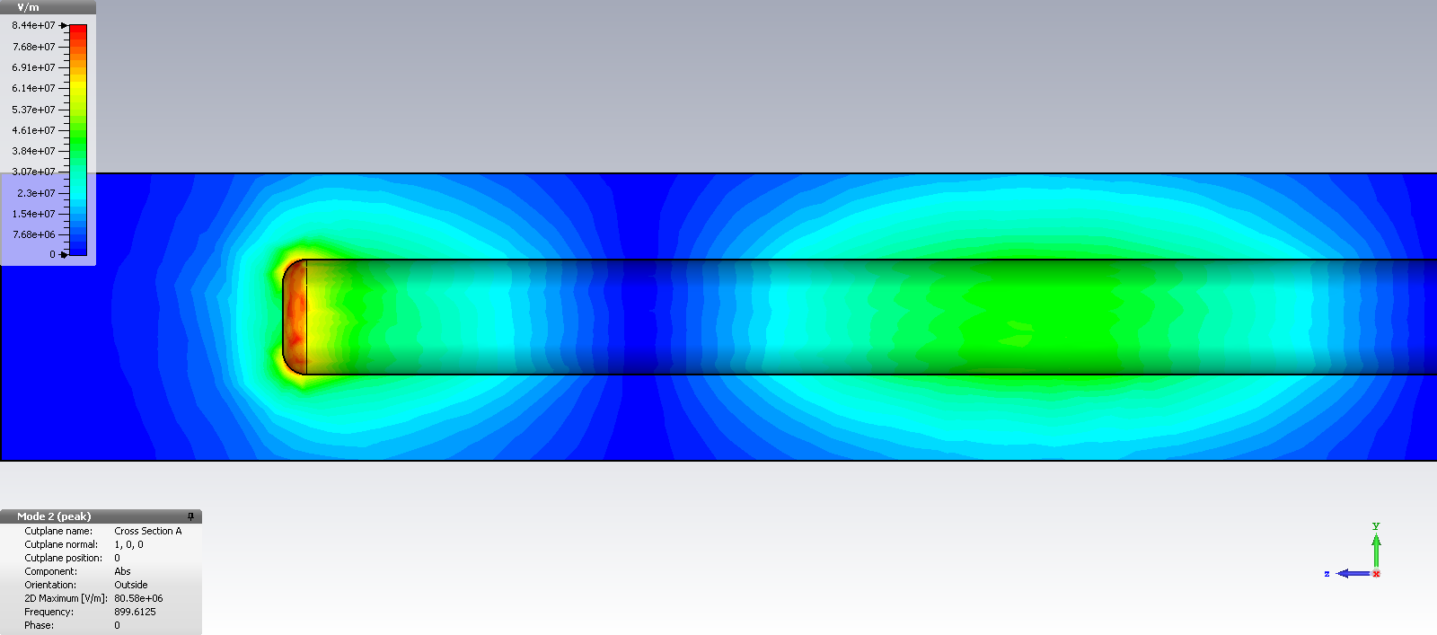
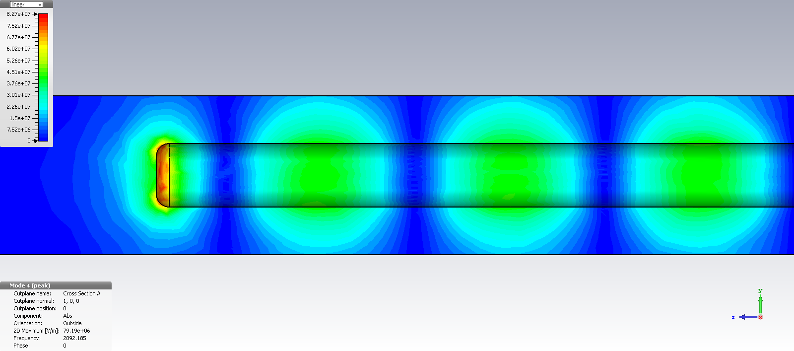
We detect that resonances occur at odd multiples of a quarter wavelength: 1, 3, 5, 7. So, the one below is at 2 + 2 + 1 = 5 quarter wavelengths.
As expected: 7 quarter wavelengths follow – and so on – until higher order non-TEM mode resonances destroy the odd-multiple of lambda/4 sequence.
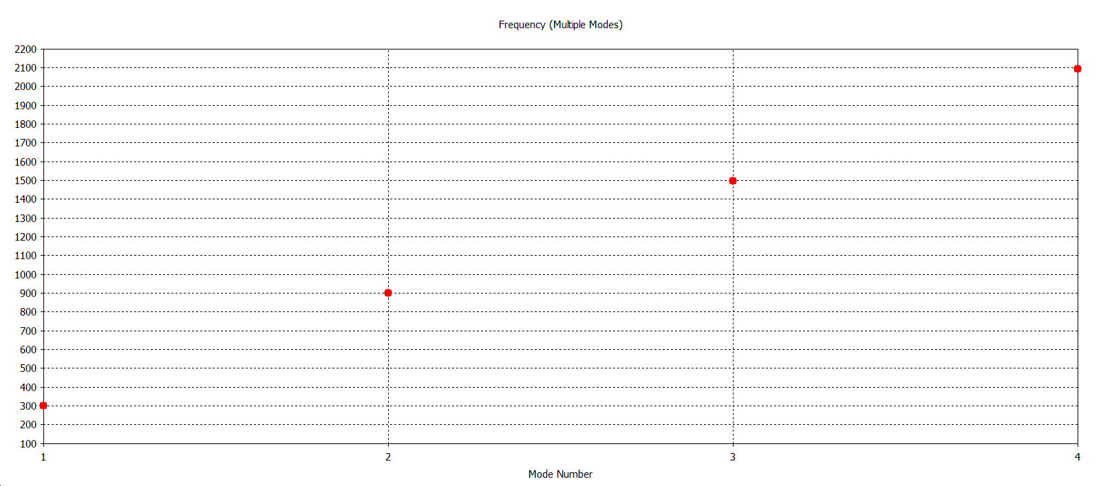
For the given rod-length of 241mm, the resonances occur at 300 MHz, 900 MHz, 1500 MHz, 2100 MHz and so on.
Dependancy of unloaded Q characteristic impedance of TEM-mode transmission line
If the rod radius of a TEM-mode quarterwave resonator is varied while keeping the outer cylinder radius constant, the well-known relationship between the unloaded Q and the resonator impedance¹ can be obtained via Eigenmode simulation.
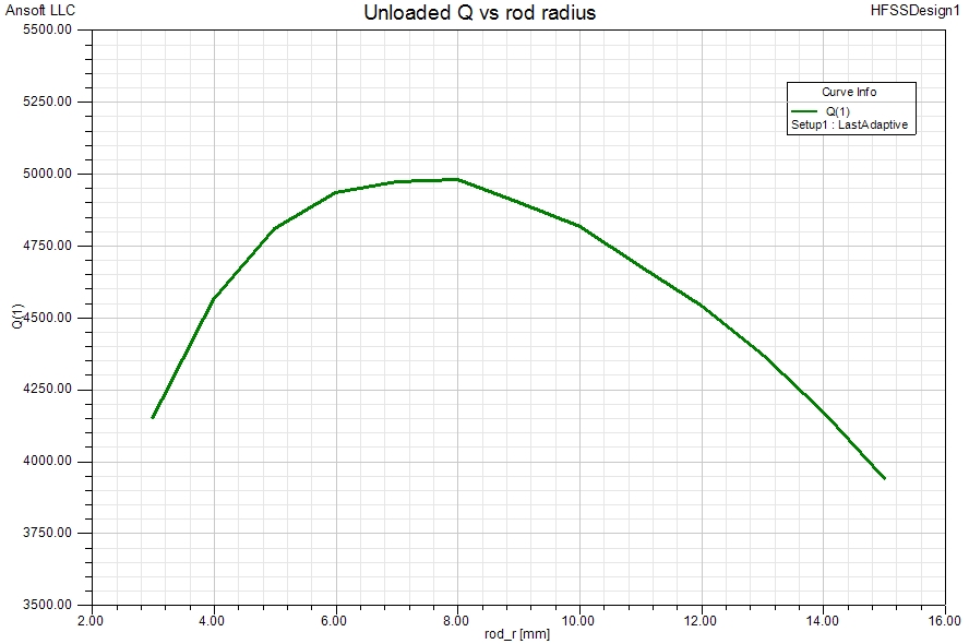
The distinct Q-maximum in the graph above shows that the ratio of stored energy to the dissipated energy per cycle is at a maximum when optimum resonator dimensions exist. Literature often suggests that a TEM-mode resonator impedance of around 70Ω is giving maximum unloaded Q. This value is based on Q formulas for idealised, pure-TEM-mode resonators. Eigenmode analysis has no such limitation and can provide reliable Q data for any type of resonator.
¹ By resonator impedance we mean here the characteristic impedance of a transmission line having the same cross-section as the resonator
Analysis of coupling between resonators
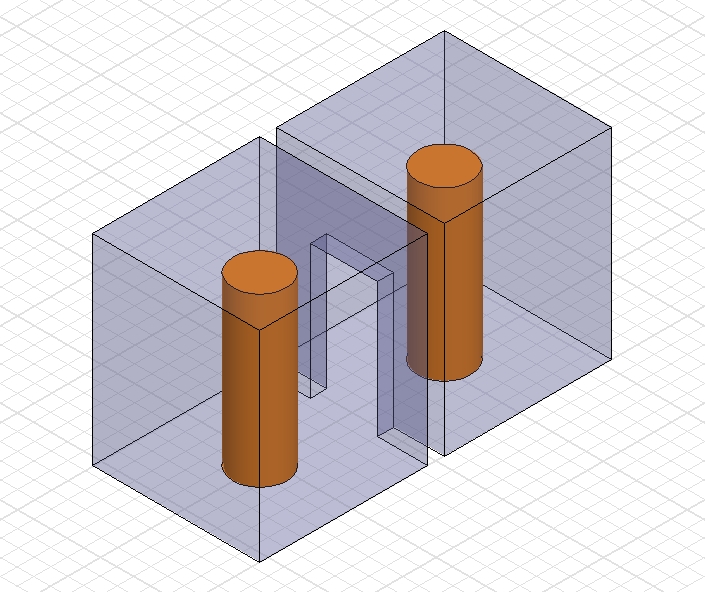
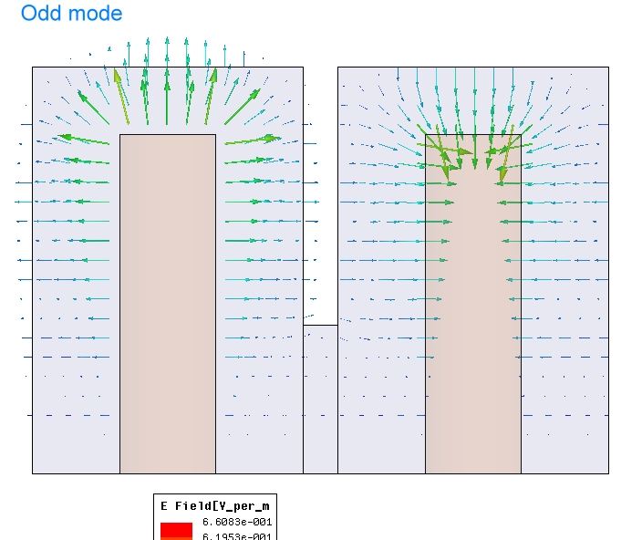
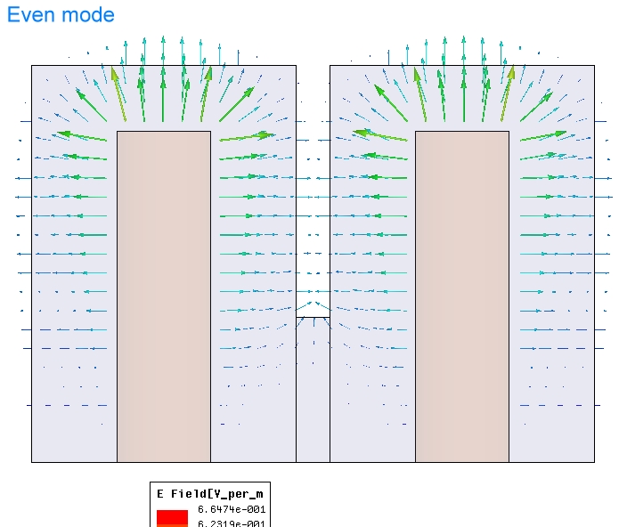
When two identical resonators are coupled by some means (aperture, loop, probe), then the resulting structure exhibits two natural modes of vibration. In the one case, both resonators are “in sync” – meaning the field vectors are identical in both resonators. In the 2nd case, there is no “sync” – instead, when field vectors in one of the resonators have a phase angle of 0 degrees, the other resonator’s field vectors are at 180 degrees (see images below).
The two Eigenmodes are indeed natural resonances of the 2-resonator structure. The Eigenmode frequencies are offset from the natural resonance of a single resonator – one Eigenmode is lower and the other is higher than the single resonator frequency. The difference between the Eigenmode frequencies of the 2-resonator structure is the coupling bandwidth (coupling coefficient x fc) with sufficient accuracy for most practical design work. Strictly, the more complex ratio of the difference and sum of the squared Eigenmode frequencies is to be used but since the difference between the two Eigenmode frequencies is usually small, the simplified calculation of the coupling bandwidth is justified. The graph below shows a typical Eigenmode result for a 2-resonator model. The width of the coupling aperture (opening of the common wall between the resonators) has been varied to see the dependency between this physical parameter and the coupling bandwidth. The y-axis unit is MHz.
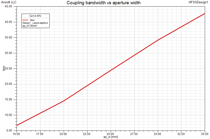
The center frequency is taken to be the geometrical mean of the two Eigenmode frequencies. The coupling opening affects the center frequency as can be seen in the graph below.
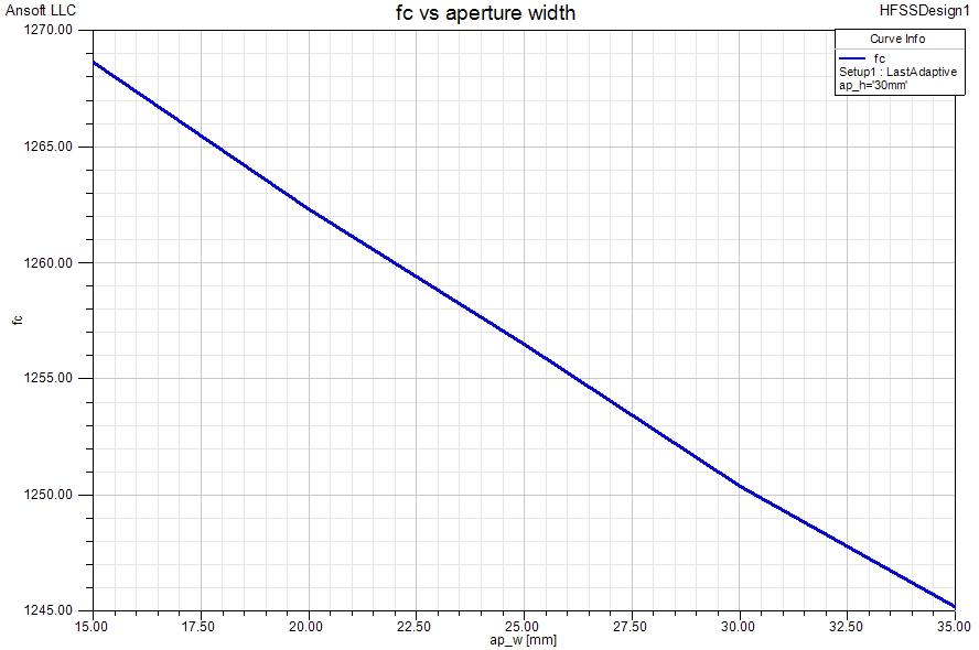
The negative slope of the graph above is perhaps best explained by considering the effect of the aperture as an inductive loading of the resonators. A larger equivalent resonator inductance leads to a lower resonant frequency.
Eigenmode analysis of couplings between two resonators necessitates full symmetry of the structure. Any lack of symmetry will lead to limited accuracy or invalid results. One way to check the effects of imperfect symmetry is to close the coupling aperture and observe the two natural modes. If these deviate significantly in frequency then the Eigenmode analysis is invalid and other methods of coupling analysis must be used. The page on planar filters contains more information on Eigenmode analysis and on alternatives to Eigenmode analysis if the latter is not available. A CST simulation data file for two coupled planar resonators can also be obtained here.
Coupled LC resonators
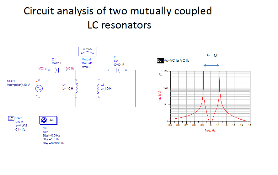
The physical TEM-mode 2-resonator structure has a lumped-element (LC) equivalence in the form of the circuit model shown below. The 2-resonator circuit also exhibits two distinct resonances that are centered around the single-resonator frequency. The offset between the two resonant frequencies depends on the strength of the coupling: strong coupling: big offset, weak coupling: small offset. We can demonstrate this by simple circuit analysis.
When two lumped element resonators with mutally coupled inductors are analysed as shown below, the voltage drop |Vc| taken across one of the resonator’s capacitors clearly shows that 2 resonant frequencies centered around the resonant frequency of the uncoupled resonator (chosen as 1Hz in this example) exist as the network’s natural modes. We can further observe that the coupling bandwidth is in this case for L=1H, C=1/(4 x PI^2), M=0.2 numerically identical to the mutual inductance (1.1 Hz – 0.9 Hz = 0.2 Hz).
Rather than just stating that the mutual coupling of two resonators creates resonances centered around fc, we show here by circuit analysis that these natural resonances exist.
Eigenmode solver stored energy
Until recently, the Eigenmode solvers of two major 3D EM simulation packages, HFSS and CST differed considerably. While CST conveniently maintain a constant stored energy of 1 Joule for Eigenmode analyses, HFSS used to normalise the Eigenmode field strength data to 1 V/m for some unknown reason. This rendered the field data of HFSS Eigenmode simulations to be of rather limited value. Since version 15 of HFSS, the Eigenmode solver stored energy is also constant and even user selectable. Insofar Ansys have followed CST’s lead in this important matter.
Other Eigenmode analysis applications
Eigenmode analysis is not limited to resonant structures. Take for example the following scenario: A coaxial line is defined. Both ends have are not waveports but we simply define that the phase difference between the E-fields at both ends is 180 degrees. The Eigenmode solver will then find all frequencies at which this boundary condition is fulfilled: all frequencies at which the length of the coaxial line is lambda/2 or a multiple thereof. This job can of course be done without an EM solver, but the example shows what an Eigenmode solver can do besides resonances and Q’s. The analysis of periodic structures can easily be done with an Eigenmode solver: it finds out where propagation exists and where not in terms of frequency bands.
IF THIS PAGE WAS USEFUL FOR YOU, PLEASE CONSIDER MAKING A DONATION. THANKS