In the second half of the 1990’s 3D Electromagnetic simulation (3D EM) become available as a simulation tool. Its application for multi-resonator filter design was initially limited due to the long calculation times involved. Electromagnetic simulation of sharply resonant filter structures with many resonators was computationally expensive – it just took too long to simulate a filter. However, together with the dramatic increase in CPU speed and by using smart design methods (Link to IEEE MTT 2003 workshop presentation) EM simulation soon progressed to becoming the key design tool for filter design and has reduced experimental design work for distributed-element and waveguide resonator filters to a minimum or made it completely redundant. The need for having a dedicated machine shop next to the filter lab certainly no longer exists. In fact ‘prototypeless design’ is a reality in many cases. Be it metallic resonator filters (like coaxial TEM-mode “combline”resonators or waveguide cavity resonators), planar (microstrip) or dielectric resonator filters, 3D EM simulators, like HFSS, CST provide all information on
- the coupling between resonators
- their n-port behavior in terms of S-parameters
- their natural resonances and associated quality factors
- their internal electromagnetic fields (power handling studies possible)
- their surface currents and surface losses (dissipative loss is considered accurately)
- their dielectric losses
- their stored energy (available via volume integration and used for Qu calculation)
In many ways, 3D EM simulation is like a ‘dream come true’ for the designer of passive rf & microwave filters. The accuracy of 3D EM simulation is so high, that usually the first hardware prototype of a filter becomes the final design product. Why is electromagnetic simulation so accurate ? The answer to this questions lies in the very nature of this type of simulation. The simulation involves the calculation of the electromagnetic fields inside the filter structure (solving of Maxwell’s equations for a given set of boundary conditions). 3D EM simulation does not use ‘equivalence’ but simulates what actually exists in nature. The subsequent access to the EM field data opens up a variety of analysis possibilities that are not available in an experimental approach. It is therefore most important that the user of EM simulation is sufficiently skilled so as to be able to exploit this versatile tool to the maximum. Such exploitation should involve processing of the analysis data. As our senior ‘filter guru’ Dr. Ralph Levy wrote in his 1999 IEEE MTT paper on the extraction of equivalent circuits: ‘… EM simulation is left to the collection of huge amounts of data’. Indeed, EM simulation creates huge files of field data. If the interest is just limited to plotting & comparing port S-parameters, then the tool is certainly underutilized. Take for example the option of being able to plot any field component along a freely defined line or curve within the structure and then perhaps process the field data in order to gain deeper insight into certain aspects of the structure. It would be a mistake to leave such possibilities unused.
Link to MW Journal 2001 article on cross-coupled filter design
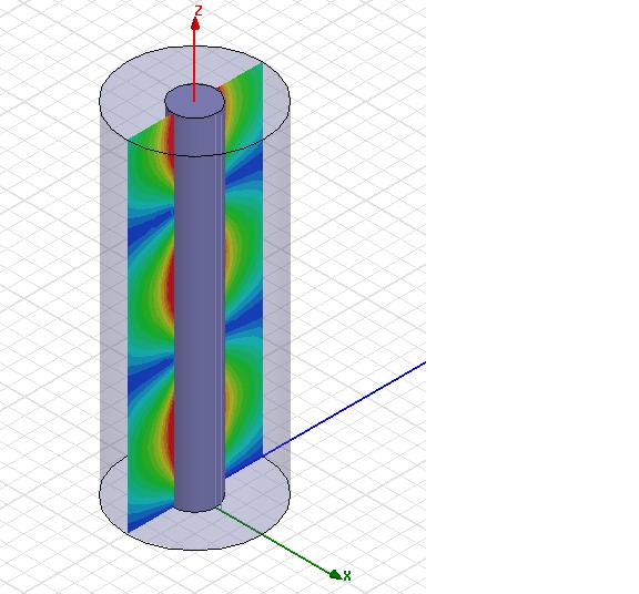
The image below shows the electric field inside a end shorted coaxial transmission line. The short circuit is at the bottom and the coaxial port is at the top. The graph shows the standing wave pattern as the E-fieldstrength magnitude on the surface of the inner conductor. The short circuit is obviously at z = 0, where |E| = 0.
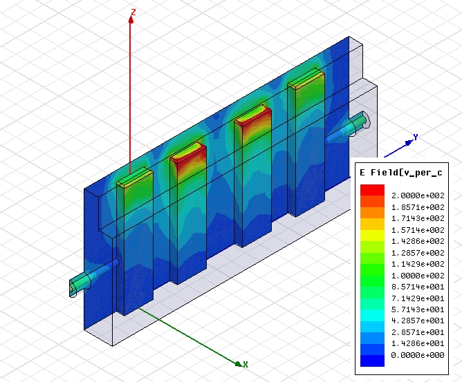
4-resonator combline filter fields at fc and port S-parameter response 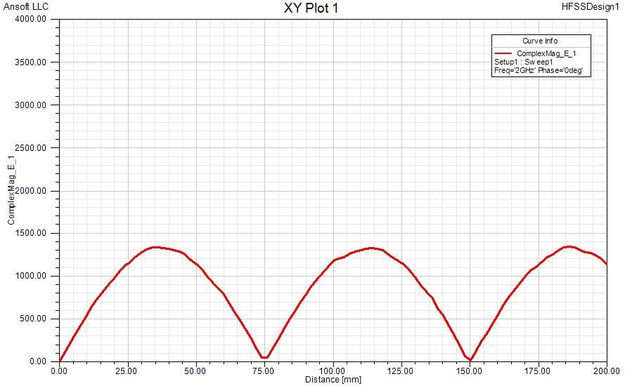
(yz-plane symmetry of the structure was used in order to minimise analysis time)
(yz-plane symmetry of the structure was used in order to minimise analysis time)

Equivalent circuit using both lumped and transmission line elements S-parameter log-magnitude responses of 3D-EM simulation and equivalent circuit simulation.

The element values of the equivalent circuit were found using the principles of space-mapping methodology. The graphs show full agreement between the ‘fine model’ (3D EM) and the ‘coarse model’ (equiv. circuit analysis). It is important to note here, that equivalent circuit element values can always be extracted from S-parameter data generated by either prototype measurement or by 3D EM simulation. Yes, 3D EM simulation analysis data can be used as if it were measured data. By comparison of extracted and nominal circuit parameters (couplings, resonator frequencies, Q’s) an accurate diagnosis of a given filter tuning status can be performed with relative ease. Furthermore, the response of the equivalent circuit with extracted element values can be optimised for fulfilling given specifications and thereby an updated ‘real-world’ equivalent circuit is obtained, leading to fast design convergence. The optimisation is here limited to those circuit element values that are indeed adjustable or variable. The specification-optimised ‘real-world’ response then becomes the updated nominal filter response. It is important to point out that 3D EM simulation does not make circuit simulation redundant. Both simulation types have their purpose and place in a filter design process.
